Value divergence at the item level
We first examined general trends towards value convergence or divergence using our value variation measure, which allowed us to estimate effects at the item level. Our results strongly supported value divergence. A mixed effects model with value variation nested in the 40 items found that timepoint has been significantly associated with greater value variation, b = 0.004, SE = 0.0007, t(239) = 5.12, p < 0.001, \(\beta\) = 0.17, 95% CIs [0.002, 0.005]. We replicated this result using a different approach in which we correlated timepoint with value variation separately for each of the 40 value items. Of the 40 values, we found that 27 have diverged over time, with a positive median correlation of 0.28 between timepoint and value variation, t(39) = 3.30, p = 0.002, Mdiff = 0.28, 95% CIs [0.11, 0.45]. Coefficients associated with each item are displayed in Fig. 1.
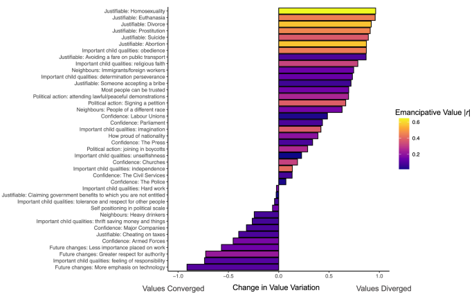
Each bar represents a correlation coefficient between timepoint and value variation for a given value (value labels are listed on the y-axis). Positive bars indicate that value variation is rising, and that values are diverging. Negative bars indicate that value variation is falling, and values are converging. The fill color indicates the absolute value of the correlation of each item with Welzel’s index of emancipative values8; brighter bars correlate either highly positively or negatively on this index.
Have certain kinds of values diverged more than others? To test this question, we measured how much each item related to Welzel’s dimensions of “sacred vs. secular” values and “emancipative vs. obedient” values8,27. Welzel developed these dimensions to differentiate between values that uphold or reject tradition and religion (sacred-secular values) from those that foster or restrict the freedom of the individual from the group (emancipative-obedient values)8. We found that a broad set of items loaded on the secular-sacred dimension, ranging from the justifiability of cheating on taxes (0.46), to the confidence in churches (0.46), to the justifiability of euthanasia (0.37). A narrower set of items loaded on the emancipative-obedient dimension. Of the examples above, only justifiability of euthanasia loaded above 0.35 (0.44).
We found that the rate of value divergence correlated with loading on the emancipative-obedient dimension, r(38) = 0.54, p < 0.001, but not the sacred-secular dimension, r(38) = 0.19, p = 0.237. This is clearly visible in Fig. 1. The 7 items with the highest divergence scores each have high loadings on the emancipative-obedient dimension. These values were (1) justifiability of homosexuality, (2) justifiability of euthanasia, (3) importance of obedience of children, (4) justifiability of divorce, (5) justifiability of prostitution, (6) justifiability of suicide, and (7) justifiability of abortion. National cultures are diverging the most on their tolerance of individual expression versus emphasis on group obedience. Supplementary Fig. 1 reproduces Fig. 1 with shading based on secular-sacred instead of emancipative-obedient loading.
Our approach allowed us to understand the nature and magnitude of divergence on emancipative values. From the first to the last timepoint, value variation across countries increased 141% for justifiability of homosexuality, 94% for justifiability of prostitution, 61% for justifiability of euthanasia, and 42% for importance of childhood obedience (Fig. 2).
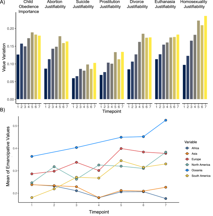
A Value variation (SD of the global distribution of normalized country means) at each WVS timepoint for the 7 items which have diverged most over time. Item labels are at the top of the figure. Bars are shaded by timepoint. B Normalized mean endorsement of the same 7 items by timepoint, with separate lines for continents. All items are coded so that higher scores reflect higher loadings on the index of emancipative values.
Divergence on emancipative values is increasingly distinguishing Western countries from non-Western ones. Consider the case of Australia and Pakistan. The first time Australians were surveyed in the WVS, 39% of participants cited childhood obedience as an important quality in children, and participants rated divorce as more unjustifiable than justifiable (0.45). When Pakistanis were first surveyed, their responses were not so different: 32% cited childhood obedience as an important childhood quality and participants rated divorce as more unjustifiable than justifiable (0.10). Over time, however, these views diverged. The last time that they were surveyed, only 18% of Australians compared to 49% of Pakistanis cited childhood obedience as an important quality, and Australians viewed divorce as much more justifiable (0.74) than Pakistanis (0.15). From the 1980s to the 2020s, similar fault lines emerged between Western and non-Western countries.
Rises in value variation for the 7 most divergent items are displayed in Fig. 2A. The clearest rises in value variation come from timepoints 1–5 and plateau across timepoints 5–7. Figure 2B illustrates changes over time in the means of these 7 values, which are aggregated to the continent level and coded such that higher values mean more emancipative values. This plot shows that Oceanic, European, North American, and South American countries have progressively endorsed more emancipative values, whereas endorsement of these values has been stable across Asian and African countries. Divergence on some values is driven by countries moving in opposite directions, as in the case of Australia vs. Pakistan on the value of childhood obedience (see Supplementary Table 16 for other examples). Other values diverged because their mean rate of endorsement changed in some countries but remained the same in others. We provide detailed methodological details about these items and countries in our Supplementary Information (e.g., Supplementary Tables 2–5).
Value divergence at the country level
We next replicated and extended these findings using our country-level value distinctiveness measure, in which we calculated each country’s deviation from the global median of each value. We first regressed this distinctiveness score on timepoint in a mixed effects model with observations nested in values, countries, and continents. This approach helped us account for the non-independence of countries within the same continent in our data analysis. Value distinctiveness has been rising over time, b = 0.003, SE = 0.0005, t(9290) = 4.98, p < 0.001, \(\beta\) = 0.05, 95% CIs [0.002, 0.004], indicating that countries have diverged in their values. We replicated this effect while controlling for spatial autocorrelation more continuously using an approach similar to the one we used to calculate value distinctiveness, b = 0.003, SE = 0.0005, t(9351) = 5.18, p < 0.001, \(\beta\) = 0.05, 95% CIs [0.002, 0.004] (see Supplementary Methods for details). This continuous method further addressed the concern that our results might have been biased by interdependence of datapoints, often called “Galton’s problem.”
Another concern is that these findings might be confounded with cohort effects, meaning that value divergence has resulted in changes in the WVS sampling strategy over time. If the cohorts of the WVS are becoming increasingly diverse, then the mean level of value distinctiveness would rise even if countries’ values stayed consistent over time. We took several steps to address this concern. First, we used centering to separate each country’s general value distinctiveness across all waves (representing a cohort effect) from its change over time from wave to wave (representing a longitudinal effect). A model including both variables found that the longitudinal effect was significant, b = 0.003, SE = 0.0006, t(10,520) = 4.92, p < 0.001, \(\beta\) = 0.04, 95% CIs [0.002, 0.004], but the cohort effect was not, b = 0.002, SE = 0.003, t(49.82) = 0.68, p = 0.503, \(\beta\) = 0.02, 95% CIs [−0.004, 0.009].
Second, we recomputed value variation and replicated our models among subsamples of countries that had less turnover and hence less susceptibility to cohort changes. We replicated value divergence among the 54 countries that participated in at least 3 waves, b = 0.003, SE = 0.0006, t(8599) = 4.82, p < 0.001, \(\beta\) = 0.05, 95% CIs [0.002, 0.004], the 32 countries that participated in at least 4 waves, b = 0.003, SE = 0.0006, t(6145) = 4.12, p < 0.001, \(\beta\) = 0.05, 95% CIs [0.001, 0.004], and the 18 countries that participated in at least 5 waves, b = 0.003, SE = 0.0007, t(4059) = 3.73, p < 0.001, \(\beta\) = 0.05, 95% CIs [0.001, 0.004]. These results provided further evidence that value divergence is not an artifact of changing sampling strategy over time, but arose from national cultures changing in diverging directions over time.
Third, we replicated the finding in sample with no turnover in sample composition—a subset of 33 countries that provided data in the 1990s, 2000s, and 2010s, which were the three decades with the greatest WVS coverage. Value distinctiveness was higher in the 2000s, b = 0.01, SE = 0.003, t(78) = 4.05, p < 0.001, \(\beta\) = 0.29, 95% CIs [0.007, 0.02], and the 2010s, b = 0.01, SE = 0.003, t(78) = 2.66, p = 0.010, \(\beta\) = 0.19, 95% CIs [0.002, 0.02], compared to the 1990s. However, we found no significant difference between the 2000s vs. 2010s, b = −0.004, SE = 0.003, t(39) = −1.41, p = 0.167, \(\beta\) = −0.10, 95% CIs [−0.01, 0.002]. This decade-based analysis provides evidence for value divergence even when we fix the country sample over time. It also suggests that value divergence has been non-linear. In our Supplementary Methods, we evaluate different non-linear models of value divergence. These models suggest that the pace of value divergence has gradually slowed over time, rather than halting at a particular point.
Analyzing value distinctiveness across countries also allowed us to estimate which countries have become most dissimilar from the rest of the world. Inglehart’s post-materialist thesis suggests that high-income countries may hold especially distinctive values, at least in the domain of morality and tolerance. However, a range of other geopolitical variables could also lead cultures to adopt distinctive social values, including wealth inequality50, distance from the equator51, globalization19, and the presence of a liberal democracy47. We accessed data on these geopolitical metrics over time, and tested whether they could predict which countries were more distinctive and which countries were less distinctive. We retained the random effects structure from our previous mixed effects models to fit these results without violating any model assumptions.
In our regression analysis, GDP per capita was the only variable that significantly predicted value distinctiveness (see Table 2), b = 0.08, SE = 0.01, t(600.59) = 8.05, p < 0.001, \(\beta\) = 0.18, 95% CIs [0.06, 0.10], with the positive coefficient indicating that higher-income countries have more distinctive values than lower-income countries. No other predictors reached significance (ps > 0.05). In our Supplementary Table 8, we show that other geopolitical variables are not significantly linked to value distinctiveness, even when we remove GDP per capita from the model.
Further analyses found that the association between GDP per capita and value distinctiveness varied across world region. Wealth was associated with value distinctiveness among European countries, b = 0.08, SE = 0.02, t(18.76) = 3.63, p = 0.002, \(\beta\) = 0.18, 95% CIs [0.04, 0.12]. However, in a regression model where we interacted GDP per capita with continent dummy-codes, we found that, compared to Europe, the effect of GDP per capita was significantly weaker in Asia, b = −0.10, SE = 0.04, t(16.66) = −2.84, p = 0.011, \(\beta\) = −0.23, 95% CIs [−0.16, −0.04], and Africa, b = −0.21, SE = 0.10, t(122.60) = −2.13, p = 0.036, \(\beta\) = −0.50, 95% CIs [−0.40, −0.02]. The association between GDP per capita and value distinctiveness was non-significant in both Africa, b = −0.14, SE = 0.10, t(109.20) = −1.38, p = 0.171, \(\beta\) = −0.32, 95% CIs [−0.32, 0.06], and Asia, b = −0.02, SE = 0.03, t(16.24) = −0.78, p = 0.448, \(\beta\) = −0.05, 95% CIs [−0.08, 0.03]. These continent comparison models were based on smaller subsets of countries, with 48 countries in the Europe vs. Asia comparison (simulated power = 80.20%) and 36 countries in the Europe vs. Africa comparison (simulated power = 98.00%). Readers should therefore interpret these findings with more caution than the tests that included the full sample of countries. Supplementary Table 13 summarizes the complete set of coefficients for these models. Our Supplementary Methods provide more details about the power analysis simulations.
Figure 3 illustrates many of the findings that we have presented in a single plot, with countries ordered along the y-axis based on their continent and on their level of value distinctiveness within continents. The x-axis illustrates each country’s value distinctiveness score at the first WVS timepoint and the final WVS timepoint, and each country’s GDP per capita is shown on the left of the y-axis. In this visualization, it is clear that most countries have diverged from the rest of the world, with more distinctive values at the final vs. the first timepoint. Second, in Western regions but not non-Western regions, divergence has been most stark for high-income countries.
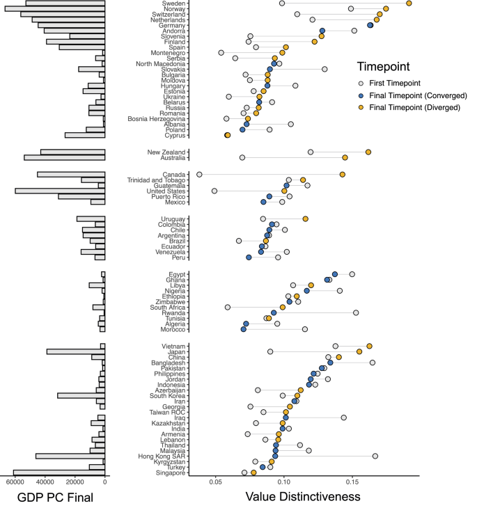
Value distinctiveness is the distance between values in a given country and the global median. Countries are organized by continent, and within continent, by value distinctiveness at the final timepoint in which the country reported data. Yellow (blue) nodes represent countries whose distinctiveness scores have increased (decreased) over time. Gray nodes represent value distinctiveness at the first timepoint. The GDP Per Capita of each country (measured at the final timepoint for each country) is displayed to the left of the plot.
These findings suggest a provocative possibility: rises in global wealth may be responsible for the worldwide divergence of values. Most countries have become wealthier over time—Western countries but also many non-Western countries like Singapore, Hong Kong, and South Korea52. This means that most countries were poorer in the earlier (vs. later) waves of the WVS. Western nations in these early waves held more emancipative values than non-Western nations, but not by a large degree. As time passed, rising wealth led Western countries to adopt more emancipative values, but it did not have the same effect for most non-Western countries. These trends led to a growing gap between high-income Western countries and the rest of the world.
Consider Hong Kong and Canada, where GDP per capita has followed a similar trend, but values have diverged. Both countries had a GDP per capita of approximately $25,000 in 2000, which doubled to approximately $50,000 by 202053,54. Over the same time interval, beliefs that homosexuality was justifiable rose in Canada from 0.49/1.00 to 0.74/1.00. Perceived justifiability of homosexuality also rose in Hong Kong, but only from 0.29/1.00 to 0.44/1.00. This means that the gap in means between Hong Kong and Canada increased by 50% during this period. One of the fastest-changing values in Hong Kong during this time was belief in children’s work ethic. From 2000 to 2021, the percent of Hong Kong participants who mentioned responsibility as an important childhood quality rose from 19% to 52%, whereas it fell from 53% to 47% in Canada.
This example shows that wealth can sometimes lead to region-specific effects on values. If rising wealth fosters emancipative values in some regions but not in others, this could explain why Western democracies have developed more distinct values over time. This would be consistent with Eisenstadt, whose “multiple modernities” thesis states that countries follow their own trajectories of modernization19. It is also consistent with Huntington’s observations that rising wealth and influence in East Asia could lead to a re-affirmation of traditional Confucian values22. Factors such as migration, political change, and decolonialization could also contribute to these trends. For example, sovereignty over Hong Kong transitioned from the United Kingdom to China in 1997, which may have affected people’s values. More research is necessary to determine the causal relationship, if any, between wealth and value change.
Within-country heterogeneity and value distinctiveness
In our next analysis, we explored whether value distinctiveness across countries was correlated with the heterogeneity of values within countries. In other words, are countries where citizens disagree on values more like the rest of the world than countries where citizens have more homogeneous values?
We calculated within-country heterogeneity using the same approach that we used to calculate value distinctiveness. But instead of taking the difference of country means from the global mean across values, we took the deviation of individual ratings from the country mean. Higher levels of within-country heterogeneity therefore represent a country with high levels of disagreement among its citizens. For example, high within-country heterogeneity in the United States might arise because liberal and conservative Americans hold very different values. In exploratory analyses, we analyzed whether within-country heterogeneity was also rising across time, signaling a divergence within countries. However, we did not find general trends in this measure. Within-country heterogeneity seems to be rising among some countries and falling among others (see Supplementary Methods).
However, we did find that within-country heterogeneity was closely linked to value distinctiveness. When we regressed value distinctiveness on within-country heterogeneity controlling for GDP per capita, Gini, globalization, political rights, and distance from equator, within-country heterogeneity robustly and negatively predicted value distinctiveness, b = −0.06, SE = 0.01, t(8,032) = −4.45, p < 0.001, \(\beta\) = −0.07, 95% CIs [−0.09, −0.03]. In other words, countries where citizens agree more on values tend to be more different from other countries. The other effects in this model remained unchanged. GDP per capita had a positive relationship and no other variables had significant associations (see Supplementary Table 12). Figure 4 visualizes the relationship between within-country heterogeneity and value distinctiveness. Our Supplementary Methods reports timepoint specific models.
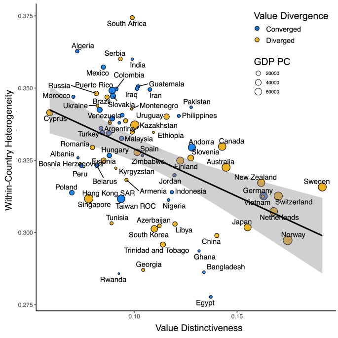
The best fit line comes from a general linear model estimate, and the shading represents the standard error centered around the best fit line. Data-point size represents GDP per capita, and datapoint fill color represents whether country values have diverged (value distinctiveness has increased) or converged (value distinctiveness has decreased) over time.
These results suggest that as countries develop more homogenous values, they may increasingly splinter from viewpoints that are shared around the rest of the world. This has happened in high-income Western nations like Sweden and Norway, where there is a higher consensus around emancipative values such as justifiability of divorce and abortion. But it has also happened in poorer nations such as China and Ghana, where consensus has formed on different values. In contrast, countries with heterogeneous values such as South Africa and India may struggle with internal division, but when averaging across their subpopulations, these countries’ values may resemble those of other countries.
What country characteristics predict value similarity over time?
In our final analysis, we explored which countries hold similar values to one another. We first fit a principal components analysis (PCA) to detect underlying dimensions in how the 40 values varied across nations. Two principal components (PCs) explained 80.70% of variation (see Materials and Methods). To understand the meaning of these dimensions, we regressed each dimension against previously developed dimensions of value variation: Welzel’s secular values and emancipative values, and Inglehart’s 12-item post-materialist index. PC1 was strongly positively linked to emancipative values, b = 0.76, SE = 0.04, t(215.60) = 19.46, p < 0.001, \(\beta\) = 0.77, 95% CIs [0.67, 0.84], and to secular values, b = 0.26, SE = 0.03, t(233.90) = 8.60, p < 0.001, \(\beta\) = 0.26, 95% CIs [0.20, 0.32]. PC2 had a smaller and less robust relationship with secular values, b = −0.13, SE = 0.07, t(194.81) = −2.10, p = 0.042, \(\beta\) = −0.13, 95% CIs [−0.27, 0.009]. No effects involving the choice index were robust (see Supplementary Methods for more information about these models).
We used these PCs as coordinates in a two-dimensional value space in which countries with similar values are closer together than nations with different values (see Fig. 5). We next fit regression models for each timepoint to test whether geopolitical characteristics could explain which countries were closer together in value space and which countries were further apart.
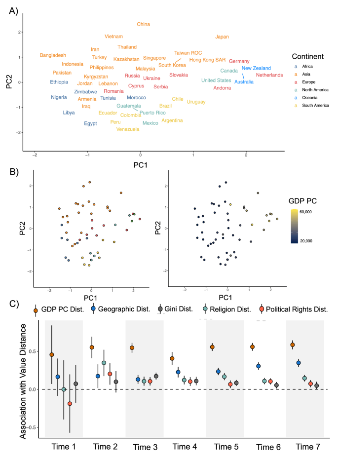
A Wave 7 country values projected on a two-dimensional space derived from a PCA of all 40 values. Proximity in this space indicates value similarity, and label color indicates continent. B A reproduction of (A) with countries as nodes colored by continent (left) and GDP per capita (right). C The association between pairwise differences in five geopolitical variables and value distance across nations, which involved n = 11 countries at Time 1, n = 20 countries at Time 2, n = 48 countries at Time 3, n = 37 countries at Time 4, n = 52 countries at Time 5, n = 54 countries at Time 6, and n = 52 countries at Time 7. Each node represents a regression coefficient, and these coefficients have been standardized so that they could be interpreted as effect sizes. Error bars are 95% confidence intervals centered around the regression coefficients.
These regressions found that wealth has been the strongest correlate of value similarity across nations over time. High-income countries share values with other high-income countries, and poor countries share values with poor countries. This effect is visible in Fig. 5 (middle right), where high-income countries like New Zealand, Germany, the Netherlands, and Japan are clustered together on the right side of the value space. We also note that the left side of the value space in Fig. 5 is denser than the right side, which replicates our prior analysis: high-income countries have developed more dissimilar values compared to the rest of the world, primarily because of their unique endorsement of emancipative values.
We also found that geographic proximity has become progressively more correlated with value similarity over time, with an effect size rising from 0.16 (Timepoint 1) to 0.35 (Timepoint 7). This is visible in Fig. 5A: high-income East Asian countries like South Korea and Singapore are closer together than high-income Western nations like New Zealand and the Netherlands. The rising predictive power of geographic proximity suggests that values are converging within regions but are diverging across regions.
Religion has also emerged as a robust predictor of value similarity. Countries with more similar religious profiles have more similar values, even controlling for their similarity in wealth, geographic position, and other geopolitical features. This finding conceptually replicates a recent analysis that found that co-religionists—even those living in similar countries—shared similar values55. The fact that values are segregating along geographical and religious fault-lines further supports Huntington’s thesis that the 21st century would see a rise of ancestral cleavages in values. By the final WVS timepoint, religious similarity and geographic proximity were stronger correlates of value similarity than having similar levels of inequality or political rights. Figure 5 plots out the associations of value similarity with each form of geopolitical similarity at each timepoint. Table 3 lists key coefficients from the value similarity regressions.

